 English
  Русский
  中文
中文  Español
  Deutsch
  Français
  Português
  Italiano
  日本語
日本語  한국어
한국어  Türkçe
  Polski
  Nederlands
  العربية
  हिन्दी
  Bahasa Indonesia
  Tiếng Việt
 Reading an OTDR trace: events, dead zones, ghosts, gainers
The OTDR draws the fibre as a line sloping down with distance and marks every place where light was lost or reflected. Reading that picture correctly — telling a splice from a bend, a ghost from a break, a real gain from a measurement artefact — is the core skill of fibre acceptance and fault location. This page explains what the instrument actually measures, how each setup parameter changes the trace, what every event type looks like and what its numbers mean, the dead-zone and dynamic-range limits, why bidirectional measurement is not optional, the standard misreadings, and how to turn a distance on the trace into a place on the route.
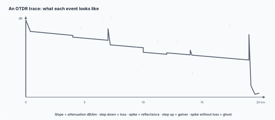
How the OTDR sees the fibre
| Mechanism | What happens | What you see |
|---|---|---|
| Pulse | a laser pulse of 5 ns to 20 µs is launched at 1310, 1550, 1625 or 1650 nm | nothing directly — the pulse is the probe |
| Rayleigh backscatter | a tiny fixed fraction of the pulse (about −79 dB at 1310 nm, −81 … −82 dB at 1550 nm for a 1 ns pulse on G.652) scatters back from every point of the fibre | the sloping line; it falls at twice the fibre attenuation because the light travels out and back, and the instrument divides by two to display one-way loss |
| Fresnel reflection | at every index step (connector, air gap, break, end) a much larger fraction returns | spikes above the backscatter line |
| Time to distance | d = c · t / (2 · n), with the group index n (IOR) of the fibre — 1.4675–1.4685 for G.652 at 1550 nm, from the fibre data sheet | the distance axis; an IOR error of 0.0015 shifts every distance by 0.1 % (10 m on 10 km) |
| Averaging | thousands of pulses are averaged; noise falls with the square root of the count | a smoother trace after 30 s to 3 min |
Setup parameters
| Parameter | Choice | Effect on the trace |
|---|---|---|
| Wavelength | 1310 + 1550 nm for loss; 1550 vs 1310 comparison for bends; 1625/1650 nm for bend hunting and for live fibre through a filter | splices look the same at all wavelengths, bends get worse with wavelength (Attenuation & windows) |
| Pulse width | short (5–30 ns) — best resolution and shortest dead zones, range under 5 km; medium (100–300 ns) — 10–40 km; long (1–20 µs) — 100–250 km with dead zones of hundreds of metres | rule: the shortest pulse that still shows the far end 6 dB above the noise; take two traces — short for the near end, long for the range; auto modes do this |
| Range | 1.5–2 × the fibre length | the end reflection and any ghosts stay on screen |
| Acquisition time | 30 s to 3 min; longer for long pulses and far ends | noise floor drops, small events become measurable |
| Index of refraction (IOR) | the fibre data sheet value; the same value for the baseline and every later comparison | distances; never "tune" IOR to make the trace match the drawing |
| Backscatter coefficient | data sheet value for the wavelength | reflectance numbers only — loss is unaffected |
| Launch and receive cords | 150–1 000 m each, longer than the attenuation dead zone of the pulse | the first and last connectors of the link become measurable |
| Thresholds | splice 0.1 dB, connector 0.5 dB, reflectance −40 dB (UPC) or −55 dB (APC), end-of-fibre 3–5 dB, section loss 0.4/0.25 dB/km | the event table flags what exceeds them |
| Live-fibre check | the instrument warns if it sees traffic light at the port | protects the OTDR receiver and confirms the fibre is dark (Safety & handling) |
Event catalogue
| Event | Signature on the trace | Typical numbers | Notes |
|---|---|---|---|
| Launch connector | large spike at 0 m followed by a dead zone | −14 … −45 dB | measure it through a launch cord; an APC launch cord gives a smaller spike |
| Fibre section | straight line sloping down | 0.33–0.35 dB/km at 1310, 0.19–0.22 at 1550, 0.20–0.24 at 1625 nm | a slope above 0.4 dB/km at 1550 means stress, water, microbending or old fibre — compare wavelengths |
| Fusion splice | small step down, no spike, the same size at every wavelength | 0.02–0.10 dB; redo above 0.15 dB | may show as a gain in one direction (see gainer) |
| Mechanical splice | small step plus a small spike | 0.1–0.5 dB, −40 … −55 dB | reflectance grows as the gel ages |
| Connector pair (UPC) | spike plus step | 0.2–0.5 dB, −45 … −60 dB | a dirty pair: bigger step, spike toward −30 dB (Endface inspection & cleaning) |
| Connector pair (APC) | step with little or no spike | 0.2–0.5 dB, below −60 dB | looks like a lossy splice — check the records |
| Macrobend | step down with no spike, much larger at 1550/1625 than at 1310 nm | 0.1–3 dB at 1550, near zero at 1310 | the wavelength dependence is the signature (Plant faults) |
| Crush, pinch, ice, tight ties | steeper slope over a section, wavelength dependent | +0.1–1 dB/km locally | often seasonal |
| Gainer | apparent step up | −0.05 … −0.3 dB | a splice between fibres with different backscatter (mode field diameter, index); the true loss is the average of the two directions |
| Exaggerated loss | the mirror image of a gainer in the other direction | +0.1 … +0.3 dB too much | same cure |
| Ghost | a spike with no loss, at twice (or a multiple of) the distance of a strong reflector, often beyond the fibre end | reflectance-like | moves or vanishes when pulse, range or launch conditions change; reduce the reflection that causes it (Reflections & return loss) |
| End of fibre, flat or UPC | large spike, then a drop into the noise | −14 … −30 dB | the classic end |
| End of fibre, APC or angled break | a drop into the noise with little or no spike | small reflectance | set end detection by loss, not by reflection |
| Break | reflective or not, then noise | any | a wet or crushed break can reflect almost nothing |
| Splitter (PON) | large step with no spike | 1:2 = 3.5 dB, 1:8 = 10 dB, 1:32 = 17 dB | needs high dynamic range; PON-optimised OTDRs exist |
| Noise floor | ragged flat tail | — | nothing beyond roughly (dynamic range − 6 dB) is measurable |
| Saturation | flat-topped spike | — | reflectance cannot be measured — use a shorter pulse or a launch cord |
| Water or hydrogen | slope increase, worst at 1383 and 1625 nm | — | multi-wavelength comparison (Reliability & ageing) |
Dead zones and dynamic range
| Pulse width | Event dead zone | Attenuation dead zone | Typical range on G.652 at 1550 nm |
|---|---|---|---|
| 5–10 ns | 0.8–1.5 m | 3–5 m | 1–3 km |
| 30 ns | 3 m | 8–10 m | 5 km |
| 100 ns | 10 m | 15–25 m | 10–20 km |
| 300 ns | 30 m | 40–60 m | 30 km |
| 1 µs | 100 m | 150–250 m | 50–80 km |
| 3 µs | 300 m | 500–700 m | 100 km |
| 10–20 µs | 1–2 km | 1.5–3 km | 150–250 km |
Values are indicative and instrument dependent. Event dead zone is the minimum distance between two reflective events that are still shown separately (the spike width 1.5 dB below its peak). Attenuation dead zone is the distance after a reflection before the trace returns to within 0.5 dB of the backscatter — a splice inside it is invisible. Dynamic range is the difference in dB between the initial backscatter and the noise level at the longest pulse and a 3-minute average; about 6 dB of it are needed for a clean measurement, so the reachable length is roughly (dynamic range − 6 dB − sum of event losses) / attenuation (Formulas & calculations).
Why bidirectional
The backscatter coefficient differs from fibre to fibre — a mode field diameter difference within the ±0.4 µm tolerance changes it by several tenths of a dB. A single-direction trace therefore reports a splice between two such fibres as too good in one direction and too bad in the other, by up to ±0.3 dB. The true loss of every splice and connector is the average of the two directions, and TIA-568.3-D Tier 2 and the IEC 61280-4 series require bidirectional averaging when splice and connector losses are reported. In practice: an OTDR with a remote unit, or two acquisitions from the two ends, and software that matches the events and averages them.
From trace distance to route position
| Factor | Effect |
|---|---|
| Fibre length vs cable length | 0.1–0.5 % excess fibre in loose tubes; the OTDR measures fibre, the drawing shows cable |
| Cable length vs sheath marks | use the metre marks recorded at both ends of each cable in the closures (Documentation & labelling) |
| Slack loops | 10–30 m stored at every closure, more at poles and building entries |
| Aerial sag | 1–3 % longer than the pole-to-pole distance |
| Duct meandering | the GIS line is shorter than the duct |
| IOR error | 0.1 % per 0.0015 of index |
Method: find the nearest known event on the trace (a closure, a panel) and measure from it, not from the instrument; convert with the recorded metre marks; confirm with a trace from the other end; use a visible fault locator or clamp-on identifier for the last metres.
Standard misreadings
| What you see | Wrong conclusion | Right reading |
|---|---|---|
| A spike beyond the fibre end | "there is more fibre" | a ghost of a strong reflector |
| A negative splice loss | "perfect splice" | a gainer — average both directions |
| No connector visible after the panel | "no loss there" | it is inside the attenuation dead zone — launch cord, shorter pulse |
| Large loss at 1550 nm only | "bad splice" | a macrobend; the splice is fine |
| High slope along a whole section | "bad fibre" | stress, water, ice or old fibre; the slope does not depend on IOR |
| Distances that disagree with the drawing by 3 % | "records are wrong" | excess fibre and slack loops — convert properly |
| Many small events near the noise | "many splices" | noise — average longer or use a longer pulse |
| The end found at 17 dB into a PON | "fibre ends at the splitter" | the end-detection threshold is too low for a splitter |
| Trace ends early with no spike | "no break, just range" | a wet or angled break — check from the other end |
| Connector reflectance reads −60 dB on a flat-topped spike | "excellent connector" | saturation — the value is meaningless |
Live fibre and PON
On a live fibre an OTDR works at 1625 or 1650 nm through a filter that blocks the traffic wavelengths in both directions. In a PON, a trace from the ONU side upward shows the drop, the splitter and the feeder cleanly; a trace from the OLT side shows all branches superimposed after the splitter and cannot separate them. Splitters need a PON-optimised OTDR with high dynamic range and short dead zones, and the distance to each splitter must come from the records (PON problems).
Reporting
Keep the native .sor file (Telcordia SR-4731) for every fibre, direction and wavelength, with the pulse, range, IOR and launch-cord length stored in it; a PDF event table is not re-analysable. The report shows bidirectionally averaged event losses, reflectances, section attenuation and total loss against the project thresholds. Under TIA-568.3-D and ISO/IEC 14763-3 the OTDR trace is the Tier 2 characterization; pass/fail of the link loss is the Tier 1 light-source-and-power-meter test (Testing & measurement, Fibre characterization).
In CodingBox
The transceivers measure the same plant from the outside: far-end Tx power minus near-end Rx power is the plant loss including everything the OTDR hides in its dead zones — the module ports and the first and last connectors. When the DDM loss exceeds the OTDR total by more than a decibel, the difference sits in those hidden places, and a bench read of the module with a clean reference cord in CodingBox tells whether the module port or the panel is the dirty one (DDM in the app, Rx power & link budget).